
Self-Explaining Neural Networks Revisited
Today’s machine learning methods are known for their ability to produce high performing models from data alone. However, the most common approaches in machine learning are often far too complex for humans to understand, hence they are often referred to as black-box models. For humans, it is impossible to understand how these models arrived at their decisions. At first glance, this does not seem to be a problem as these models perform very well in almost all application areas, sometimes even surpassing human performance. Therefore, it is not surprising that these models have been adopted in a wide range of real-world applications, especially in increasingly critical domains such as healthcare, criminal justice, and autonomous driving. However, when taking a deeper look it becomes clear that all of these applications have a direct impact on our lives and can be harmful to our society if not designed and engineered correctly, with considerations to fairness. Consequently, demand for interpretability of complex machine learning models has increased over recent years.
In this blog post we will present an extension of a Self-Explaining Neural Network (SENN) [1] in order to enhance interpretability.
Achieving Interpretability
Two different paradigms on achieving interpretability of machine learning models are predominant in the literature: post-hoc explanation methods and intrinsically interpretable models.
Post-hoc explanation methods aim to provide information on black-box models after training and do not pose any constraints or regularization enforcing interpretability on the model of interest. These methods can be divided into gradient or reverse propagation methods that use at least partial information given by the primary model, and complete black-box methods that only use local input-output behavior for explanations.
Conversely, an intrinsically interpretable approach aims to make a model interpretable by its formulation and architecture and thus takes into account interpretability already during training. A first and natural approach to achieve model interpretability is to restrict oneself to the use of simple and often close to linear (regression like) models that can be understood by humans on a global level. Other approaches aim to induce sparsity in the context of a neural network. Lastly and most relevant for the approach taken here, we want to mention explanation generating models. These models produce explanations which are at the same time used for predictions and thus aim to be intrinsically interpretable by network architecture.
Self-Explaining Neural Networks
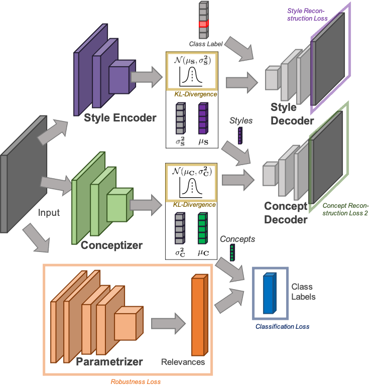
Figure 1: Architecture of a Self-Explaining Neural Network
In this work, we use an explanation generating architecture called Self-Explaining Neural Network from David Alvarez-Melis and Tommi Jaakkola [1].
A SENN consists of two components: a conceptizer $h(x)$ and a parametrizer $\theta(x)$. The conceptizer aims to encode input data as meaningful concepts while the parametrizer learns explanations which weigh the concepts for the prediction task. Hence, a SENN aggregates concepts and explanations using the inner product such that we can write the prediction as $f(x) = \langle h(x), \theta(x)\rangle$.
The design of both components is crucial for attaining interpretability and the authors propose different requirements on each of them. The parametrizer should be locally interpretable, meaning that if inputs $x_0$ and $x_1$ are close to each other, then $\theta(x_0)$ and $\theta(x_1)$ should not differ significantly. For this purpose, the authors propose a loss that enforces the parametrizer to follow a Lipschitz-like continuity property. In particular, they add the following term to the minimization objective:
which is high (and consequently penalizes more) if the derivative of the whole SENN with respect to the input $x$ differs greatly from the derivative of a SENN with fixed parametrizer. For more details please have a look at the original paper [1].
Three desiderata are stipulated for the conceptizer:
- grounding (human-interpretable concepts)
- diversity (non-overlapping concepts), and
- fidelity (relevance of concepts).
Alvarez-Melis and Jaakkola propose the use of an autoencoder for the conceptizer. We think this approach does not per se full-fill any of the above stated desiderata:
- human interpretability of encodings can suffer e.g. from discontinuities in the latent space of the autoencoder,
- although autoencoders compress raw inputs to a lower dimensional space, these embeddings may still contain information irrelevant to the prediction task, and
- autoencoders do not guarantee disentangled representations.
In this blog post we want to focus on the first two points listed above. A crucial part for human interpretability of a SENN depends on the robustness of the conceptizer itself. That is, the conceptizer should also be relatively stable for close inputs with the same class label (similar to the local interpretability requirement demanded on the parametrizer). Moreover, the model should be as interpretable as possible for the user. In particular, the user should not have to use some subjective heuristic to filter out concepts that are irrelevant to the prediction task. Thus, we want to learn concepts that only contain information required for prediction. Therefore, we are proposing to use a new architecture based on variational autoencoders for the conceptizer.
Brief Introduction: Variationonal Autoencoder (VAE)
If you are already familiar with variational autoencoders just skip this section and head straight to the next. Otherwise what follows is a brief and hopefully easy to understand introduction to variational autoencoders.
As the name suggests, variational autoencoders are closely related to autoencoders. As a form of nonlinear principal component analysis (PCA) [6], autoencoders try to compress information inherent in an input image $x$ into a lower dimensional representation $z$. Variational autoencoders embed this idea in a bayesian variational setting. Here, we assume that any input data $x$ is a random variable generated by some lower-dimensional latent factors (also random variables) $z$. This implies that we can write the likelihood of our data $x$ as $p_\theta(x) = \int p_\theta(x|z) p(z)$.
The conditional likelihood $p_\theta(x|z)$ is usually modeled using a neural network parametrized by $\theta$. This neural network $p_\theta(x|z)$ is referred to as the decoder. Further, $p(z)$ is the prior over $z$ taken to be a standard Gaussian in the following. Ideally, we would like to find $\theta$ that maximizes the data likelihood $p_\theta(x)$. Unfortunately, in general, both computing the data likelihood $p_\theta(x)$ and computing the true posterior $p_\theta(z|x)$ is infeasible due to the required marginalization.
This brings us to the centerpiece of a VAE: the Evidence Lower BOund or ELBO. To get there we need to take two steps:
- Variational approximation: Since finding the true posterior $p_\theta(z|x)$ is in general intractable, the VAE uses an encoder $q_\phi(z|x)$ (usually a neural network) to approximate the true posterior.
- Bounding likelihood from below: Next, the data log-likelihood $p(x)$ can be rewritten by inserting the variational approximation $q_\phi(z|x)$ from point 1 in such a way that we end up with a lower bound that is easy to maximize:
where in the first equation we have used that densities integrate to one, in the second we used Bayes theorem, in the third we inserted a multiplicative one, in the fourth we used the definitions of expectation and KL-divergence, and for the last inequality the fact that any KL-divergence is always greater or equal to $0$.
Let us look at the three terms before the inequality in more detail:
- The first term can be interpreted as a reconstruction term that is high if we are able to generate reconstructions (the output of the decoder $p_\theta(x|z))$ that are close to our original input $x$.
- The second term is a regularization term that encourages our variational posterior $q_\phi(z|x)$ to be close to our prior (if we assume the variational posterior to belong to a gaussian family and take the standard gaussian as a prior this has a closed form solution - yay)
- The third term is the variational error term. Since we cannot compute the true posterior $p_\theta(z|x)$ explicitly the variational error term also cannot be computed. We can, however, say that this term must be greater or equal to $0$. Hence by removing it from the equation we arrive at a lower bound for the log likelihood.
Side note: it is interesting to see that the lower bound derived above is tight when our variational posterior $q_\phi(z|x)$ is equal to the true posterior $p_\theta(z|x)$ (i.e. when the KL-divergence between these two distributions approaches $0$).
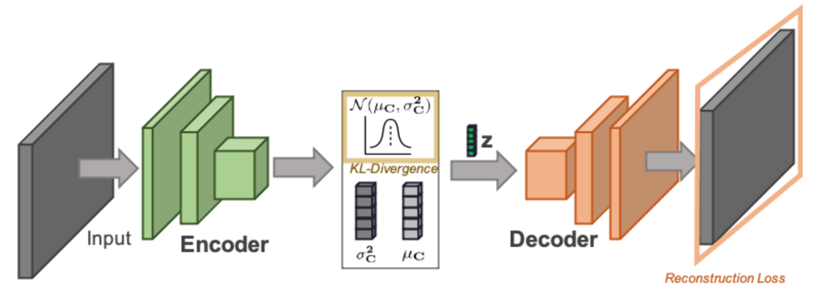
Figure 2: Variational Autoencoder
As already hinted at above, in practice encoder $q_\phi(z|x)$ and decoder $p_\theta(x|z)$ are often modeled by two neural networks composed as in the network architecture depicted in Figure 2.
$\beta$-VAE
Finding latent factors $z$ that explain variation in the data can already be a big step towards interpretability. The learned latent representations are often low dimensional and thus easier to visualize. For interpretability it would be even more helpful if the single components of the latent representations were independent of each other. In a best case scenario each component should capture one visible factor of variation. For example, when applying a VAE on a dataset containing human faces we would like one component of the latent representation to capture hair color, another one eye color, and so on. In the probabilistic setting this translates to a posterior $q_\phi(z|x)$ that factorizes along each of its dimensions.
To encourage disentanglement among components of $z$, [2] introduce a new hyperparameter $\beta$ that weighs the KL-divergence term in the ELBO. The ELBO of $\beta$-VAE then becomes $\log p_\theta(x) \geq \mathbf{E}_{q_\phi(z|x)} \log p_\theta(x) - \beta\, D_{KL}(q_\phi(z|x)\;|\;p(z))$. Higher $\beta$ encourages the posterior $q_\phi(z|x)$ to be closer to the prior which is factorizable in case of a standard Gaussian. Thus, higher $\beta$ should also encourage the posterior to be factorizable and in turn lead to more disentanglement among the single components of the latent representation $z$. In practice almost always a $\beta$-VAE is used with $\beta$ being a crucial hyperparameter to be tuned.
VaeSENN

Figure 3: Architecture of the proposed VaeSENN
In order to address the shortcomings of the SENN model mentioned early, we propose a new model with a revised architecture of the conceptizer named VaeSENN. The VaeSENN (see Figure 3), uses supervised autoencoders [3] implemented via a $\beta$-VAE. The idea is to use two-stage autoencoding to separately encode parts of the input irrelevant and relevant to the prediction task. A first supervised variational autoencoder learns embeddings for those parts of the input data not relevant to the prediction task (e.g., style or rotation in handwriting). In the following, we refer to this first autoencoder as the style autoencoder and to the learned embeddings as styles. Encoded styles are then given as additional input to a second variational autoencoder (the conceptizer in the framework of a SENN) which learns concepts used for the prediction task.
The use of a supervised $\beta$-VAE in both autoencoders addresses all three shortcomings of autoencoders mentioned in the introduction. First, the variational approach enhances continuity of the latent space and thus hopefully also human interpretability. Second, the variational approach with a factorizable prior in both autoencoders enhances disentanglement of styles but more importantly also of concepts. Third, the additional input of styles allows the conceptizer to learn relevant encodings since it does not have to embed information irrelevant to the prediction task.
In order to learn styles (the task of the style autoencoder), we run a $\beta$-VAE on the inputs with one crucial addition: we will not only give the embeddings produced by the style encoder to the style decoder but also the label of each instance (i.e., we add one-hot encoded labels to the style decoder’s input). This supervision procedure follows supervised adversarial autoencoders presented in [3], with the difference that we do not use a Generative Adversarial Network but a KL-divergence loss to enforce a prior distribution on the latent space. Using a supervised $\beta$-VAE we are not only enforcing disentanglement within the latent space but also disentanglement of label information from all other latent factors of variation.
In the second stage, the same architecture is used to learn concepts. Again, the input images are processed by a probabilistic encoder $q_\phi(z|x)$. However, instead of additionally including the label information, we now give the style information learned during the first stage to the concept decoder. In this way, concepts are disentangled from all other latent factors regarding information irrelevant to the prediction task (styles). Equally important, the use of a $\beta$-VAE for the conceptizer also encourages disentanglement between concepts.
Experiments
Now that we have laid out our approach for VaeSENN in more detail it is time to evaluate it on some real datasets. In the beginning of this blog post we promised to improve the conceptizer in a SENN by enhancing grounding (human-interpretablity) and diversity (non-overlap) of concepts. Thus, we will now elaborate in more detail on achieved interpretability with respect to continuity of the latent space and on disentanglement of latent factors.
As datasets we used MNIST and CIFAR10. We found that MNIST worked best for comparing visualization of concepts due its limited complexity. To distinguish performance we found that it was useful to run experiments on a more complex data set, namely CIFAR10.
For hyperparameter settings and other training configuration details see the implementation on our github page.
Accuracy
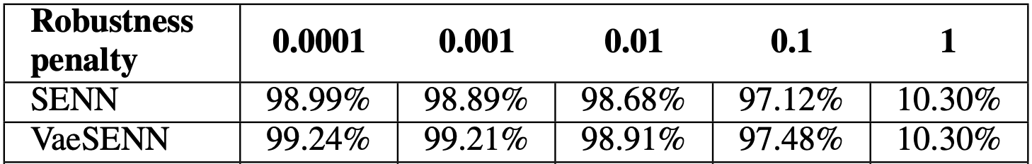
Table 1: Test accuracy on MNIST
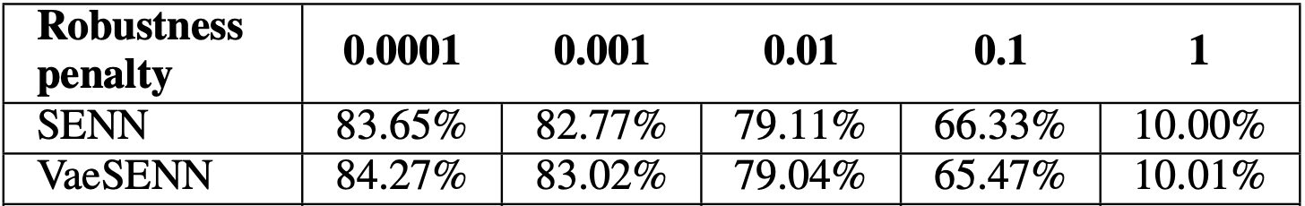
Table 2: Test accuracy on CIFAR10
We evaluated test accuracy of the above specified models on MNIST and CIFAR10 for robustness penalties ranging from $\lambda = 1 \times 10^{−4}$ to $\lambda = 1 \times 10^{0}$. Tables 1 and 2 show that VaeSENN has test accuracies comparable to a SENN. Thus, in the following we will focus on arguing that our proposed models achieve enhanced interpretability while achieving similar accuracy compared to a SENN.
Grounding of Concepts
To analyze grounding of concepts we first assess the continuity of the latent space using two visualization techniques: principal component analysis [6] and t-distributed stochastic neighbor embedding (t-SNE) [7]. With using two distinct visualization techniques we hope to reduce the risk of coming to conclusions that result from the specific characteristics of the visualization technique rather than from the concepts themselves. Figure 4 shows the results of visualizing 4000 learned concepts on a test data set for SENN and VaeSENN.
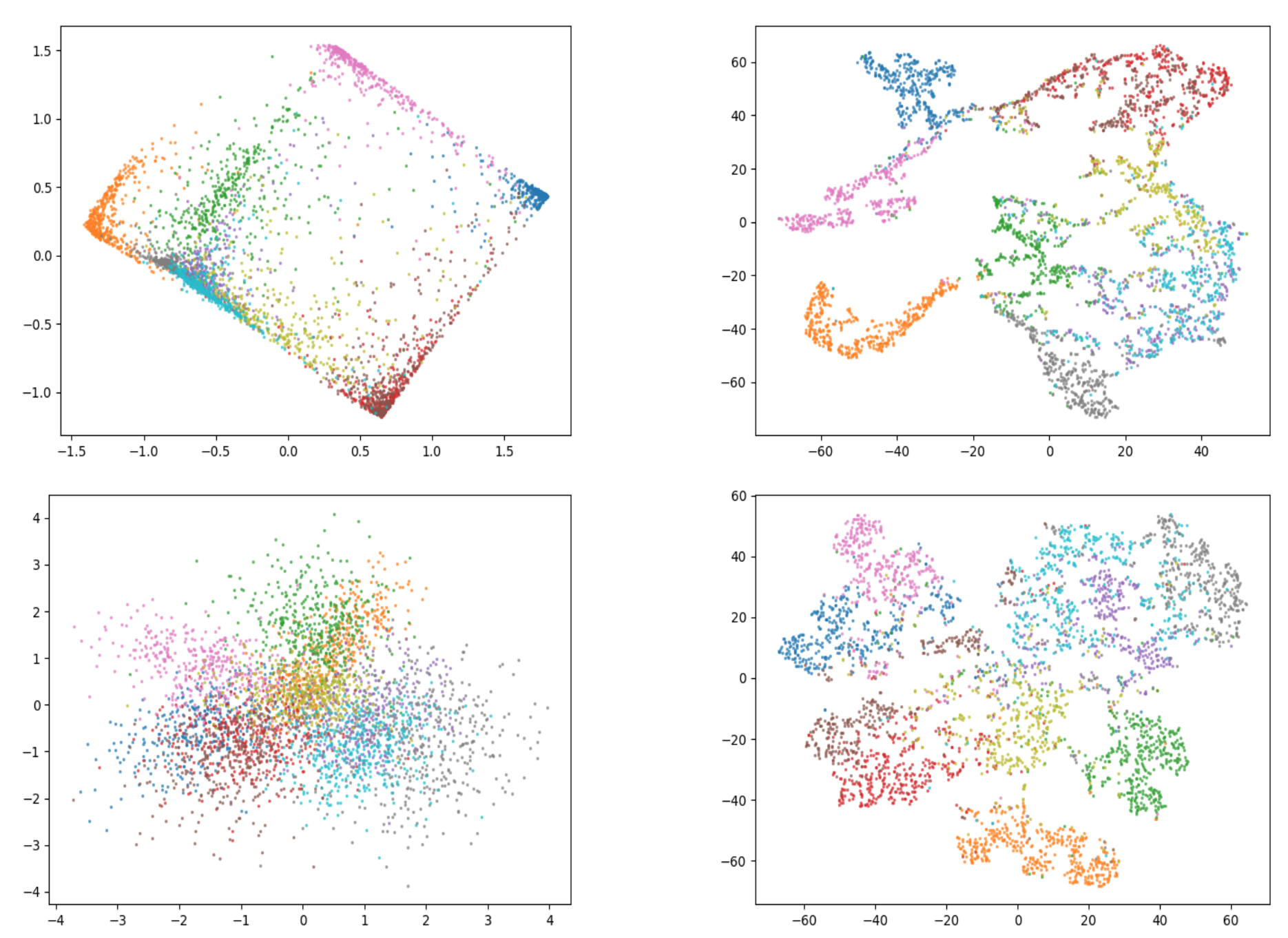
Figure 4: Visualization of concepts in latent space for SENN, and VaeSENN on MNIST. Rows: The first row shows results for SENN, the second for VaeSENN. Columns: The first column uses PCA as a visualization method, the second t-SNE.
It can clearly be seen that the latent space for VaeSENN is of much nicer shape than that for SENN. Due to the use of a variational component in VaeSENN this is not surprising. Especially the PCA plot for SENN indicates some discontinuities within the latent space. Overall, the use of a variational part within the conceptizer substantially increased interpretability of concepts by improving the continuity of the latent space.
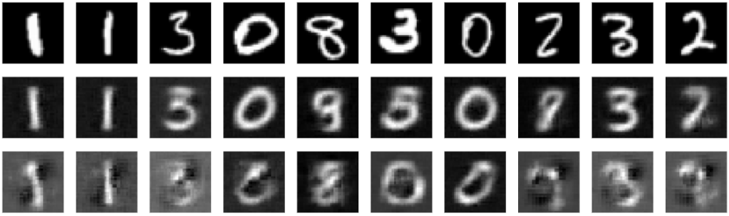
Figure 5: Sampling from latent space in SENN: the first row shows the original input image, the second row shows the decoded image without added noise, and the third row shows the decoded image with added noise.
Another possibility to analyze interpretability of the latent space is to sample from it and see if the decoded samples resemble meaningful pictures. For a SENN and a VaeSENN we encoded 10 images randomly chosen from the test data set. We then perturbed concept vectors by adding gaussian noise. Resulting decoded images can be seen in Figure 5 and 6 for SENN and VaeSENN respectively. Sampling from the latent space for a VaeSENN visibly works better than for a SENN which is in line with our previous finding that the latent space of the former also is more continuous.
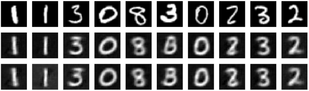
Figure 6: Sampling from latent space in VaeSENN: the first row shows the original input image, the second row shows the decoded image without added noise, and the third row shows the decoded image with added noise.
Diversity of Concepts
Due to the distinct characteristics between the latent space of a SENN and VaeSENN, disentanglement is harder to compare. On an absolute basis, Figure 4 shows that VaeSENN is clearly able to learn concepts that are disentangled by class (while not being disentangled too much which could jeopardize continuity of latent space). Evaluating disentanglement of concepts in this way might be an over-simplification. Further, no clear superiority of VaeSENN in terms of diversity can be seen. Thus, we will make some comments on how to better learn and evaluate disentanglement in the discussion.
Visualization of Styles
Lastly, we want to take a look at whether the style part of a VaeSENN actually learns what it promises. For the first stage of a VaeSENN we claimed that the style autoencoder learns different styles of an image of the same class. On MNIST we would expect this to be rotations or line thickness of handwritten numbers. To verify our claim we conducted the following experiment: a style vector with all entries except for one is set to zero and a class label was given to the style decoder. We then varied the non-zero entry of the style vector in a range from -2 to 2. Decoded images are shown in Figure 7. Indeed, the first and third row seem to show rotation of a number and the second the location of the horizontal line of a four (ranging from high to low from left to right).
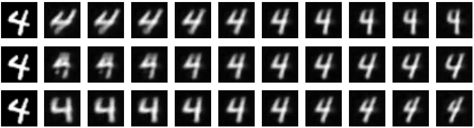
Figure 7: Images sampled from the latent space of the style encoder manipulating a single dimension of the latent space (we arbitrarily chose ”4”) .
Discussion
The idea of a SENN to break up a potentially huge neural network into parts that can be interpretable generally seems promising and certainly has its finger on the pulse of the times where demand for interpretability is on the rise. A SENN alone, however, will most likely not do the job.
Most importantly, interpretability crucially depends on the disentanglement of concepts which is a whole different area of research in itself. Thus, we think a stronger focus has to be put on learning latent representations whose components are independent of each other e.g. via Factor VAE [4] and henceworth also on measuring achieved disentanglement (some empirical evaluation methods have been introduced in [2] and [5]).
For more details on our project please visit our github page.
References
[1] D. Alvarez-Melis and T. S. Jaakkola, “Towards robust interpretability with self-explaining neural networks,” 2018.
[2] I. Higgins, L. Matthey, A. Pal, C. Burgess, X. Glorot, M. Botvinick, S. Mohamed, and A. Lerchner, “beta-vae: Learning basic visual concepts with a constrained variational framework,” in ICLR, 2017.
[3] A. Makhzani, J. Shlens, N. Jaitly, I. Goodfellow, and B. Frey, “Adversarial autoencoders” 2016.
[4] H. Kim, A. Mnih, “Disentangling by Factorising” 2019.
[5] F. Locatello, S. Bauer, M. Lucic, G. Rätsch, S. Gelly, B.Schölkopf, and O, Bachem, “Challenging Common Assumptions in the Unsupervised Learning of Disentangled Representations” 2019.
[6] H. Hotelling, Analysis of a Complex of Statistical Variables Into Principal Components. Warwick & York, 1933.
[7] L. van der Maaten and G. Hinton, “Visualizing data using t-sne,” Journal of Machine Learning Research, vol. 9, no. 86, pp. 2579–2605, 2008.