Exploring Siamese Networks for Self-Explaining Neural Networks

In our last post we have talked about Self-Explaining Neural Network (SENN) from David Alvarez-Melis and Tommi Jaakkola [1] and extended the model by a new conceptizer based on supervised $\beta$-variational autoencoders (VaeSENN). As mentioned in the last post, with a VaeSENN we aimed to overcome the following shortcomings of an autoencoder used by Alvarez-Melis and Jaakkola for the conceptizer in a SENN:

1. human interpretability of encodings can suffer e.g. from discontinuities in the latent space of the autoencoder,
2. although autoencoders compress raw inputs to a lower dimensional space, these embeddings may still contain information irrelevant to the prediction task, and
3. autoencoders do not guarantee disentangled representations.

While a VaeSENN addresses all of these issues, [4] correctly point out that a crucial part of interpretability for a SENN depends also on the robustness of the conceptizer itself. That is, the conceptizer should also be relatively stable for close inputs with the same class label (similar to the local interpretability requirement demanded on the parametrizer). Thus, it should for example not be possible to slightly change the image of a four and obtain concepts corresponding to an image of a five.

In this blog post we will present another extension of a Self-Explaining Neural Network [1] in order to enhance interpretability-robustness while keeping all other properties of a VaeSENN.

Siamese Networks

Before diving into our model we will briefly discuss Siamese networks. If you are already familiar with Siamese networks just skip this section and head straight to the next.

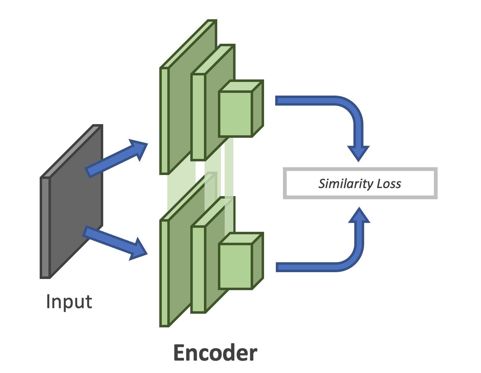
Figure 1: Architecture of a Siamese Network

Siamese networks are a class of neural networks that consist of two (or more) identical subnetworks that share parameters and weights. The aim of these networks is to evaluate the similarity of different inputs by comparing latent representations, which is why these networks are used in many applications including signature and face verification, one-shot learning, and others.

A main problem of Siamese networks is that they have a tendency towards collapsing solutions. For example: imagine our goal is to train a Siamese network to determine whether two different images from MNIST represent the same digit or not. We could train a Siamese network consisting of two different subnetworks with pairs of images from the same class and minimize the Euclidean distance between the two feature vectors as a loss. The problem is that the network could set all input weights to zero. By doing so the network collapses to a constant solution which minimizes the Euclidean distance but would never detect images from different classes. Therefore, we need to subject the training of Siamese networks to certain conditions to avoid collapsing solutions.

One possibility to avoid collapsing solutions is to use a contrastive loss. A popular example of such a loss is the triplet loss. A triplet loss is a loss function where an anchor input is compared to a positive input (in-class example) and a negative input (out-class example). The distance from the anchor input to the positive input is minimized, and the distance from the anchor input to the negative input is maximized.

For more details on training Siamese networks with a contrastive loss have look at [5].

VSiamSENN

We introduce a Siamese network architecture, named VSiamSENN, to learn embeddings invariant to in-class noise, and thus, enhancing interpretability-robustness. A triplet loss is used to ensure that embeddings corresponding to images of the same class are mapped close to each other while images of a different class are explicitly mapped far away from each other. Further, in order to better shape the latent space we additionally use a variational scheme comparable with $\beta$-VAE. In that sense, the training objective here slightly differs from [2]: while [2] aims to learn informative embeddings in a lower-dimensional space we aim to learn an informative posterior distribution of embeddings in this lower dimensional space.

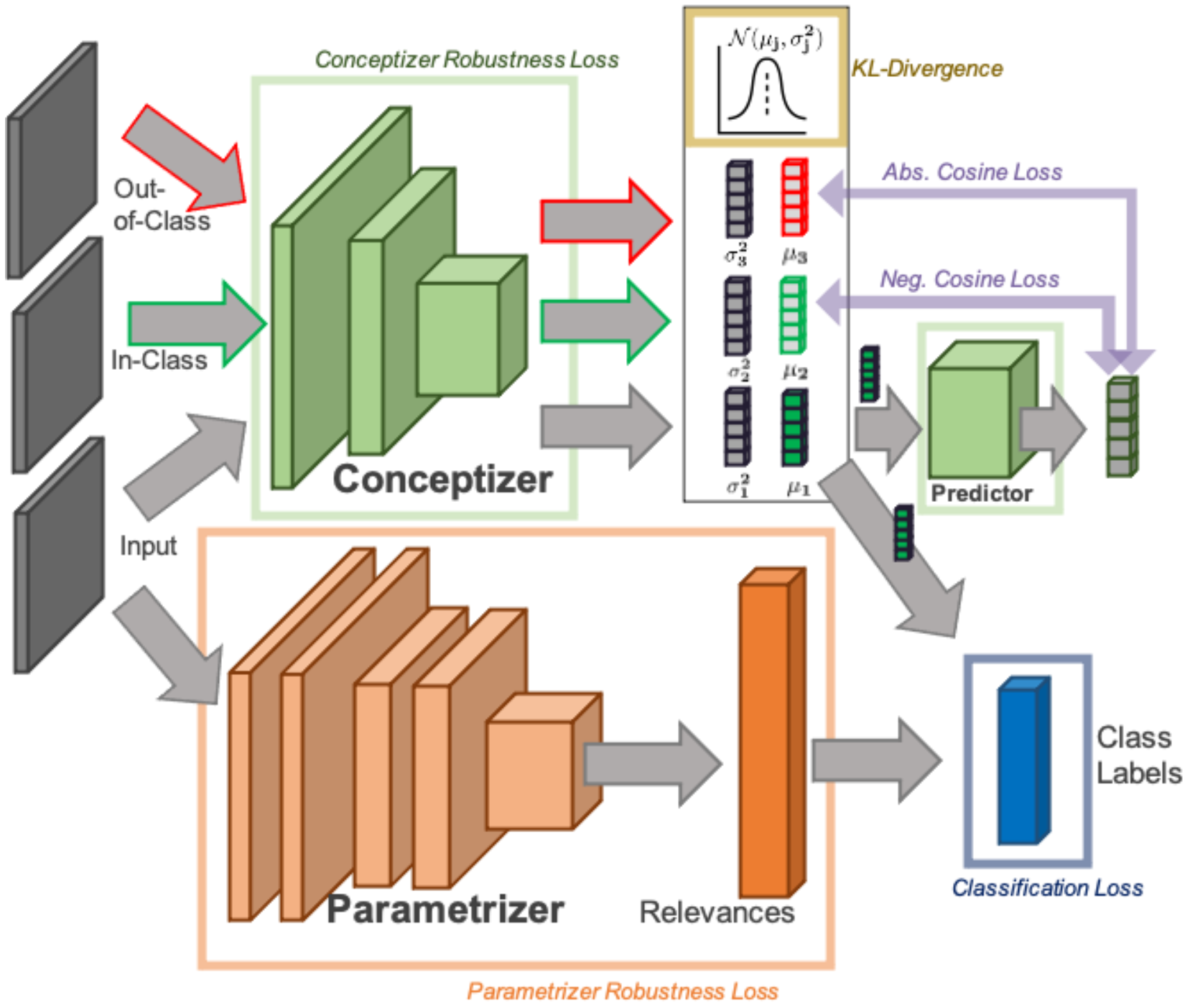
Figure 2: Architecture of VSiamSENN

The proposed network architecture (Figure 1) and training procedure is described in the following. During training our architecture takes as an input three images:

1. the image $x_1$ to be classified,
2. in-class example $x_2$, a sampled image of the same class, and
3. out-of-class example $x_3$, a sampled image of a different class.

The three images are processed by the same probabilistic encoder $q_{\phi}(z|x)$ (the conceptizer in the SENN framework).

[2], [3] use a predictor $g$ for estimating the expectation of the latent encoding over the space of data augmentations by minimizing the negative cosine distance to its estimated expectation. Our approach differs, in that the predictor $g$ instead estimates the expectation of the posterior mean corresponding to all images of the same class by minimizing negative cosine distance between sampled latent encodings from the posterior distributions and expected posterior mean of images of the same class. Additionally, to ensure class separation in the latent space, the absolute cosine distance between sampled latent representations from the posterior distributions and expected posterior means of images of different classes is minimized. We define negative cosine distance for two inputs $x_i$ and $x_j$ with $i,j \in {1,2,3}$:

$$ \begin{align*} \mathcal{D}(z_i, \bar{\mu_j})&= -\frac{z_i}{||z_i||_2}\cdot \frac{\bar{\mu}_j}{||\bar{\mu}_j||_2}\qquad \end{align*} $$

where $z_i$ is a sample drawn from the posterior distribution $q_{\phi}(z|x_i)$ with mean $\mu_\phi(x_i)$ and $\bar{\mu}_j=g(\mu_\phi(x_j))$ is the estimated expectation of the posterior mean.

In order to better shape the latent space, a KL-divergence loss is used to enforce a prior distribution (a unit Gaussian) on the latent space. Moreover, as suggested in [4], we introduce a new local-Lipschitz stability property for $\mu_\phi(x_1)$ with respect to $x$, in order to ensure that small changes in the input do not cause significant changes in concepts. This leaves us with the following loss to be minimized:

$$ \begin{align*} \mathcal{L}&=\frac{\mathcal{D}(z_1, \bar{\mu}_2)}{2}+\frac{\mathcal{D}(z_2, \bar{\mu}_1)}{2}+\frac{|\mathcal{D}(z_1, \bar{\mu}_3)|}{2}+\frac{|\mathcal{D}(z_3, \bar{\mu}_1)|}{2}\notag\\ &\quad +\beta \cdot \left[ \frac{\mathbb{D}_{KL}(q_\phi(z_1|x_1)||p(z))}{3}+\frac{\mathbb{D}_{KL}(q_\phi(z_2|x_2)||p(z))}{3}\right.\notag\\ &\quad\left.+\frac{\mathbb{D}_{KL}(q_\phi(z_3|x_3)||p(z))}{3}\right]+ \eta \cdot ||\nabla_{x_1}\, \mu_\phi(x_1)||_2\notag\\ &\quad +\lambda \cdot \underbrace{\mathcal{L}_{\theta}(f)}_{\text{Robustness Loss}}+\underbrace{\mathcal{L}_{y}(f(x_1), y_1)}_{\text{Classification Loss}} \end{align*} $$

Experiments

In the previous blog post we compared a SENN to a novel architecture, called VaeSENN, that uses a variational approach in order to learn label relevant and non-relevant features. There, we focused on grounding and disentanglement of learned concepts in particular. Here, we will instead concentrate on robustness of interpretability.

For hyperparameter settings and other training configuration details see the implementation on our github page.

Accuracy

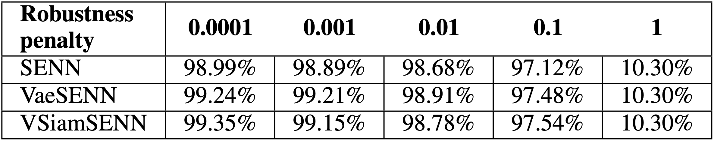
Table 1: Test accuracy on MNIST

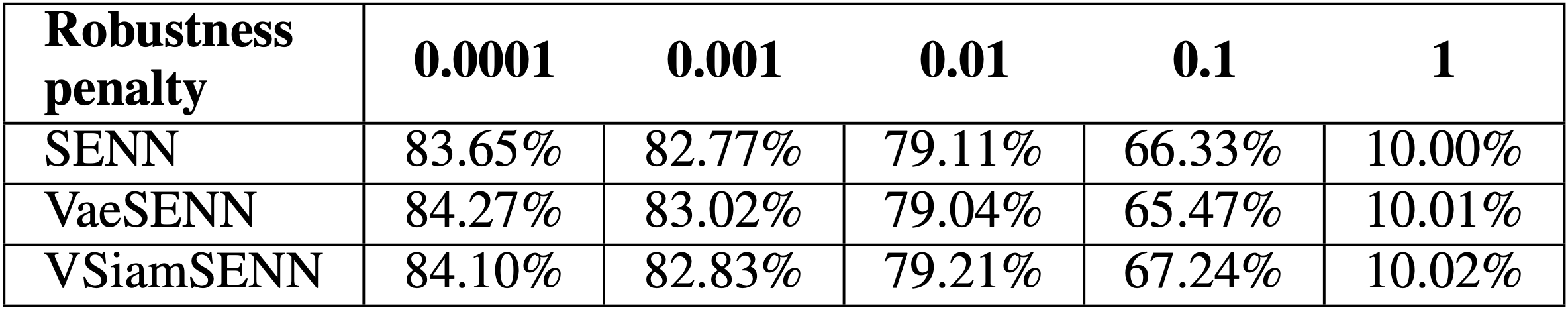
Table 2: Test accuracy on CIFAR10

We evaluated test accuracy of a SENN and a VSiamSENN on MNIST and CIFAR10 for robustness penalties ranging from $\lambda = 1 \times 10^{−4}$ to $\lambda = 1 \times 10^{0}$. Experimental results of VaeSENN are depicted as well, thus we can assess the performance of all three approaches. Tables 1 and 2 show that test accuracies across models lie in a similar range and cannot serve as a metric of comparison. In the following we will focus on arguing that our proposed model achieves enhanced interpretability while achieving similar accuracy compared to a SENN.

Grounding and Disentanglement of Concepts

To analyse the structure and characteristics of learned concepts we use two visualization techniques: principal component analysis [6] and t-distributed stochastic neighbor embedding (t-SNE) [7]. Figure 2 shows the results of visualizing 4000 learned concepts on a test data set for SENN and VSiamSENN.

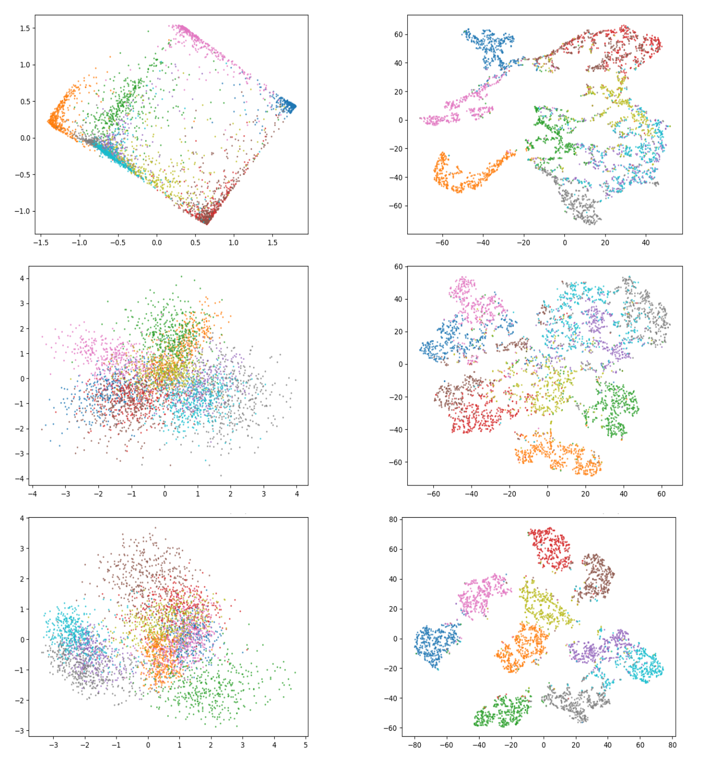
Figure 2: Visualization of concepts in latent space for SENN, VaeSENN and VSiamSENN on MNIST. Rows: The first row shows results for SENN, the second for VaeSENN, the third for VSiamSENN. Columns: The first column uses PCA as a visualization method, the second t-SNE.

The PCA suggests that the latent space defined by the concepts learned with VSiamSENN is smoother than that defined by the concepts learned with a SENN. Further, the t-SNE plot shows that the latent representations generated by a VSiamSENN and a SENN are both disentangled by class labels. To be able to evaluate and compare a VSiamSENN and a SENN in more detail, in the following, we will quantify the robustness of interpretability.

Interpretability-Robustness

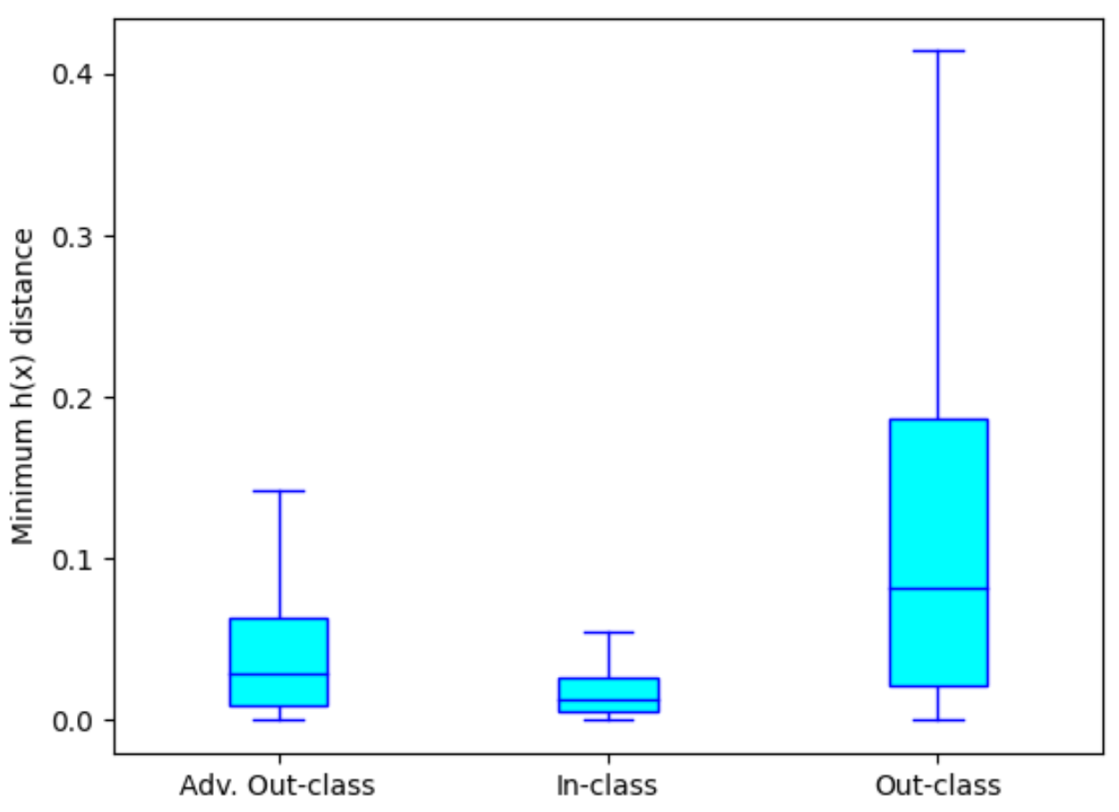
Figure 3: Comparison on the distribution of adv. out-class, in-class and out-class distance for SENN on MNIST dataset with accuracy 98.89% $(\lambda = 1 × 10^{−3})$.

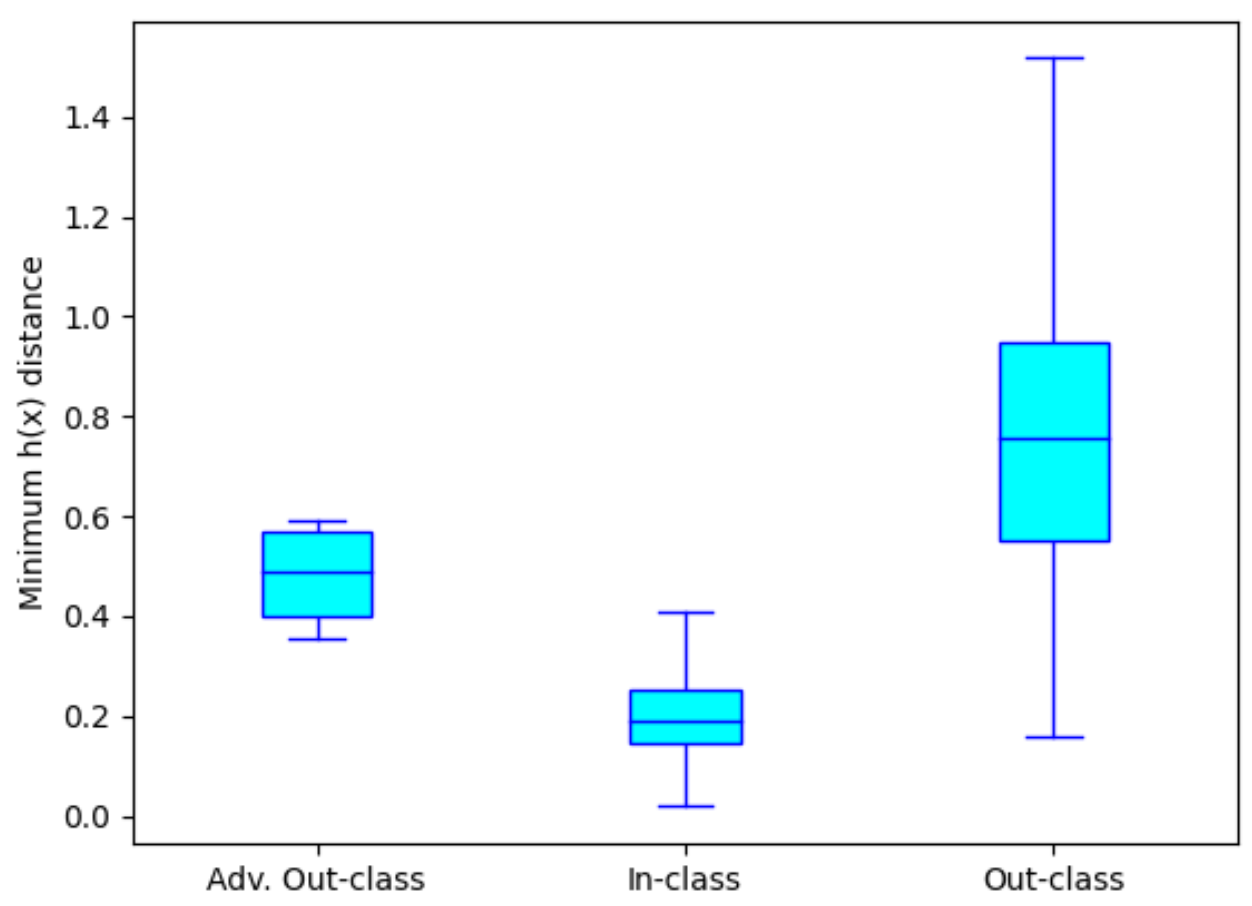
Figure 4: Comparison on the distribution of adv. out-class, in-class and out-class distance for VSiamSENN on MNIST dataset with accuracy 99.03% $(\lambda = 1 \times 10^{−3}, \eta=1 \times 10^{−4})$.

For concepts to be interpretable with respect to a class prediction small changes in input images should not cause significant chances in concepts while the model output stays the same i.e. concepts should be robust. To measure this robustness we will use three metrics introduced in a paper on interpretability robustness of a SENN [4]. For a given training point $x$ the three metrics we will use in the following are:

1. in-class distance: the smallest distance between the concept of the given data point and another data point belonging to the same class (this should be small).
2. out-class distance: the smallest distance between the concepts of the given data point and another data point belonging to a different class (this should be large).
3. adversarial out-class distance: the smallest distance of the concepts of an image close to our input image (having the same class) and concepts of images belonging to other classes than the input image (in case you are interested in adversarial attacks: we use PGD attack [9] and measure closeness with an $L_\infty$- ball of size $\epsilon = 0.2$).

As shown in Figure 3 for a SENN we observe that in-class distance is smaller than out-class distance. More importantly, we observe that adversarial out-class distance is similar to in-class distance. In comparison, for the VSiamSENN (Figure 4) we observe that the adversarial out-class distance as well as the out-class distances are significantly larger than in-class distance. The results imply that adversarial perturbations are often succesful in changing concepts of an image to concepts of an image belonging to a different class in a SENN but rarely for a VSiamSENN.

Discussion

While a SENN as originally proposed in [1] does not necessarily fulfill all desiderata stated for robust interpretability (see last post) it gives rise to a ”plug-in” principle that could be used to build custom models with enhanced interpretability. The separation of conceptizer and parametrizer within a SENN allows to plug in different architectures and pose different interpretability requirements on each of them. In this post and the last one, we showed two possible examples for such a ”plug-in” to enhance interpretability where including a variational element seemed to be especially advantageous. There is still much room for improving the interpretability of a SENN and we are keen to see where this field of research is heading.

For more details on our project please visit our github page.

Authors

Edward Günther, Massimo Höhn, and Carina Schnuck

References

[1] D. Alvarez-Melis and T. S. Jaakkola, “Towards robust interpretability with self-explaining neural networks,” 2018.

[2] X. Chen and K. He, “Exploring simple siamese representation learning,” 2020.

[3] J.-B. Grill, F. Strub, F. Altche, C. Tallec, P. H. Richemond, E. Buchatskaya, C. Doersch, B. A. Pires, Z. D. Guo, M. G. Azar, B. Piot, K. Kavukcuoglu, R. Munos, and M. Valko, “Bootstrap your own latent: A new approach to self-supervised learning,” 2020.

[4] H. Zheng, E. Fernandes, and A. Prakash, “Analyzing the interpretability robustness of self-explaining models,” 2020.

[5] R. Hadsell, S. Chopra, and Y. LeCun, “Dimensionality reduction by learning an invariant mapping,” In CVPR, 2006.

[6] H. Hotelling, Analysis of a Complex of Statistical Variables Into Principal Components. Warwick & York, 1933.

[7] L. van der Maaten and G. Hinton, “Visualizing data using t-sne,” Journal of Machine Learning Research, vol. 9, no. 86, pp. 2579–2605, 2008.

[8] L. van der Maaten and G. Hinton, “Visualizing data using t-sne,” Journal of Machine Learning Research, vol. 9, no. 86, pp. 2579–2605, 2008.

[9] A. Madry, A. Makelov, L. Schmidt, D. Tsipras, and A. Vladu, “Towards deep learning models resistant to adversarial attacks,” 2019.